R for beginners | part 2
Youtube playlist for this tutorial series https://www.youtube.com/playlist?list=PLn-5J2322iDh2Rf6BUR836bAkYTXHB65O
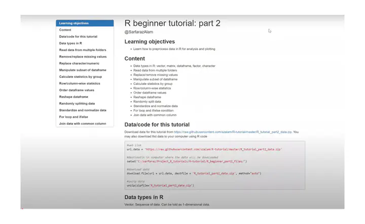
Learning objectives
- Learn how to preprocess data in R for analysis and plotting
Content
- Data types in R: vector, matrix, dataframe, factor, character
- Read data from multiple folders
- Replace/remove missing values
- Manipulate subset of dataframe
- Calculate statistics by group
- Row/column-wise statistics
- Order dataframe values
- Reshape dataframe
- Randomly split data
- Standardize and normalize data
- For loop and if/else condition
- Join data with common column
Data/code for this tutorial
Download data for this tutorial from https://raw.githubusercontent.com/szalam/R-tutorial/master/R_tutorial_part2_data.zip. You may also download thd data to your computer using R code
#web link
url.data = 'https://raw.githubusercontent.com/szalam/R-tutorial/master/R_tutorial_part2_data.zip'

#destinatin in computer where the data will be downloaded
setwd('C:/sarfaraz/Project_R_tutorials/R-tutorial/R_beginner_part2_files/')

#download data
download.file(url = url.data, destfile = 'R_tutorial_part2_data.zip', method="auto")

#unzip data
unzip(zipfile='R_tutorial_part2_data.zip')
Data types in R
Vector: Sequence of data. Can be told as 1-dimensional data.
#Vector
v1 = c(1,2,3,4)
v2 = c('A', 'B', 'C', 'D')

print(v1)
## [1] 1 2 3 4
print(v2)
## [1] "A" "B" "C" "D"
Matrix: 2-dimensional data with row and columns. Data type (or class) of all the matrix element should be same (numeric, character)
#Matrix. All values are numeric
m = matrix(1:10, nrow = 5, ncol = 2)
m
##      [,1] [,2]
## [1,]    1    6
## [2,]    2    7
## [3,]    3    8
## [4,]    4    9
## [5,]    5   10
Dataframe: 2-dimensional data with row and columns. Data type of different columns can be different. One column can be numeric and another can be character.
#Dataframe. Column 1 and 2 numeric, and column 2 character
c1 = c(1:5)
c2 = c(11:15)
c3 = c('A', 'B', 'C', 'D', 'E')
df = data.frame(c1, c2, c3)
List: Similar to 3-dimensional data. For example, a list with two objects (or lists) can have dataframe in the first list and vector in the second list. It can store different types of objects in different list.
#Lists
l = list()
l[[1]] = df
l[[2]] = v1
str(l)
## List of 2
##  $ :'data.frame':    5 obs. of  3 variables:
##   ..$ c1: int [1:5] 1 2 3 4 5
##   ..$ c2: int [1:5] 11 12 13 14 15
##   ..$ c3: chr [1:5] "A" "B" "C" "D" ...
##  $ : num [1:4] 1 2 3 4
Factor: Used to categorize data. Can be integer or character. Factor is very usefull during categorical plots.
setwd('C:/sarfaraz/Project_R_tutorials/R-tutorial/R_beginner_part2_files/data1/')
df = read.csv('rainfall_data.csv')
head(df)
##        Date Month Year      loc_A       loc_B       loc_C
## 1 1/15/1981     1 1981 188.682179 83.57845383 164.6300596
## 2 2/15/1981     2 1981  83.090653 42.52718642  46.4600436
## 3 3/15/1981     3 1981 136.694246 99.88195830 130.9438164
## 4 4/15/1981     4 1981  40.223348          NA  37.0420120
## 5 5/15/1981     5 1981  46.528754 13.56783115  18.1241447
## 6 6/15/1981     6 1981   4.081162  0.01092273   0.1125636
#lets plot year vs rainfal in loc_A in the original dataframe 'df'
df.mod = df[!is.na(df$loc_A),]
#plot(df.mod$Year,df.mod$loc_A)

#convert the Year column of df into factor
df.mod2 = df.mod
df.mod2$Year = as.factor(df.mod2$Year)
# plot(df.mod2$Year,df.mod2$loc_A)
Read data from multiple folders
A commonly used technique to read csv/txt files from different folders is shown below. Here, we read one .csv file from folder “data1”" and 1 .txt file from folder “data2”.
fold1 = 'C:/sarfaraz/Project_R_tutorials/R-tutorial/R_beginner_part2_files/data1/'
fold2 = 'C:/sarfaraz/Project_R_tutorials/R-tutorial/R_beginner_part2_files/data2/'

#read csv from folder data1
df1 = read.csv(paste0(fold1,'rainfall_data.csv'))
df2 = read.table(paste0(fold2,'d1.txt'),fill =T)
Remove/replace missing values
Here we read a csv file with missing data (which is generally read as “NA” in R). Then remove/replace NA values.
#set working directory
setwd('C:/sarfaraz/Project_R_tutorials/R-tutorial/R_beginner_part2_files/data1')

#read rainfal data
df = read.csv('rainfall_data.csv')
summary(df)
##      Date               Month            Year          loc_A
##  Length:144         Min.   : 1.00   Min.   :1981   Min.   :  0.0393
##  Class :character   1st Qu.: 3.75   1st Qu.:1984   1st Qu.: 11.8359
##  Mode  :character   Median : 6.50   Median :1986   Median : 42.6371
##                     Mean   : 6.50   Mean   :1986   Mean   : 73.8314
##                     3rd Qu.: 9.25   3rd Qu.:1989   3rd Qu.:112.1323
##                     Max.   :12.00   Max.   :1992   Max.   :416.9089
##                                                    NA's   :3
##      loc_B               loc_C
##  Min.   :  0.01092   Min.   :  0.0719
##  1st Qu.:  2.93055   1st Qu.:  5.6136
##  Median : 17.68898   Median : 27.4605
##  Mean   : 34.57416   Mean   : 55.3813
##  3rd Qu.: 50.15615   3rd Qu.: 80.5734
##  Max.   :245.07228   Max.   :342.1296
##  NA's   :3           NA's   :2
#calculate mean
mean(df$loc_A)
## [1] NA
mean(df$loc_A, na.rm = T)
## [1] 73.83143
#find ids of NAs for loc_A, loc_B, loc_C
id.na.a = which(is.na(df$loc_A)==T)
id.na.a = which(is.na(df$loc_A)==T)
id.na.a = which(is.na(df$loc_A)==T)

#replace NA with -999
df[id.na.a,4] = -999

#remove rows with NA values in loc_A
df2 = df[-id.na.a,]

#another way to remove rows with NA in a single line
df3 = df[!is.na(df$loc_A),]
Similar to rows, specific column can also be removed from the dataframe
#removing column 2 from df
df.rm = df[,-2]

#removinb column 2 and 3
df.rm.2 = df[,c(-2,-3)]
Replace character/numeric
Replacing character/numeric value is a neccesary is skill. For example, a data may have spelling mistake (“Californiaa”" instread of “California”). Here, we will learn how to replace character/numreic values.
#set working directory
setwd('C:/sarfaraz/Project_R_tutorials/R-tutorial/R_beginner_part2_files/data1')

#read data and check unique Regions
df.tmp = read.csv('replace_char_num.csv')
unique(df.tmp$Region)
## [1] "California" "Ohio" "Nevada" "Californiaa"
#looks like there is a spelling mistake. "Californiaa" should be "California". Lets correct it
df.tmp[df.tmp$Region == 'Californiaa',] = 'California'
unique(df.tmp$Region)
## [1] "California" "Ohio" "Nevada"
Using ifelse function can be an efficient way to do the replacing job.
#here we will replace Region Ohio with Washington. The code replace where region is Ohio, otherwise keep as it is.
df.tmp$Region = ifelse(df.tmp$Region == "Ohio", "Washington", df.tmp$Region)
unique(df.tmp$Region)
## [1] "California" "Washington" "Nevada"
The method I showed above are also applicable for numeric values or signs. For example, you might want to replace numeric values, or signs like “#” or “?” or even blank spaces " “. The above codes are extremely useful for data cleaning and preparation for analysis.
Manipulate subset of dataframe
I will show three ways to select part of a dataframe that follow user-specified condition. Let us separate data with months 1,3 and 7
#method 1: identify the indices, then separate
id.tmp = which(df$Month == 1 | df$Month == 3 | df$Month == 7)
df.new1 = df[id.tmp,]

#method 2: using %in%
mon.tmp = c(1,3,7)
df.new2 = df[df$Month %in% mon.tmp,]

#method 3: using filter funtion of the library dplyr. Call dplyr library first
library(dplyr) # if you don't have the library than install using install.packages('dplyr')
##
## Attaching package: 'dplyr'

## The following objects are masked from 'package:stats':
##
##     filter, lag

## The following objects are masked from 'package:base':
##
##     intersect, setdiff, setequal, union
df.new3 = filter(df, Month == c(1,3,7))
#to select subset within a range (2 to 8)
df.new4 = filter(df, Month <=8 & Month >=2)
Let us multiply 1.5 with all the rainfall in month 2 and 4 that occurred in loc_A
#identify the indices of rows with month 2 and 4
id.tmp = which(df$Month == 2 | df$Month == 4)

#multiply 1.5 with the loc_A column having row id as id.tmp
df[id.tmp,4] = df[id.tmp,4] * 1.5
Calculate statistics by group
Let us calculate mean rainfall in all the January months (month = 1).
#using aggregate function
df.gr1 = aggregate(df[,c(4,5,6)],by = list(df[,2]),FUN = mean,na.rm = T)
head(df.gr1)
##   Group.1     loc_A     loc_B      loc_C
## 1       1  26.42661 59.006145  85.862767
## 2       2 202.93061 65.025331 104.953206
## 3       3 168.03628 91.019927 136.666929
## 4       4 -49.59144 28.554692  45.024609
## 5       5  36.71198 10.733013  19.447401
## 6       6  17.97584  4.148091   7.806769
Row/column-wise statistics
Calculate mean value of all rows/columns
#calculate mean along selected columns (here, column 4, 5 and 6)
df.gr2.mean = apply(df[,c(4,5,6)], 2, mean,na.rm = T) # here 2 means column-wise

#also calculate column-wise standard deviation
df.gr2.sd = apply(df[,c(4,5,6)], 2, sd,na.rm=T)

#calculate row-wise mean in selected columns (here, column 4, 5 and 6)
df.gr3 = apply(df[,c(4,5,6)], 1, mean,na.rm = T) # here 1 indicate row
# we can also do this using colMeans() and rowMeans() functions
df.gr2_2 = colMeans(df[,c(4,5,6)], na.rm =T)
df.gr2_2
##    loc_A    loc_B    loc_C
## 55.74019 34.57416 55.38134
df.gr3_2 = rowMeans(df[,c(4,5,6)], na.rm =T)
Order dataframe values
Let us sort the datframe in ascending/descending order
#sort in ascending order
df.tmp = df[order(df$loc_A),]
head(df.tmp)
##           Date Month Year         loc_A      loc_B        loc_C
## 88   4/15/1988     4 1988 -1498.5000000 60.2571635  77.04603099
## 11  11/15/1981    11 1981  -999.0000000 50.1490205 162.31109130
## 49   1/15/1985     1 1985  -999.0000000 28.2914828  26.01976957
## 8    8/15/1981     8 1981     0.0393286  0.5085948   0.16317945
## 103  7/15/1989     7 1989     0.1020899  0.2536141   0.07192623
## 68   8/15/1986     8 1986     0.1706050  0.8371909   0.50209573
#sort in descending order
df.tmp2 = df[order(-df$loc_A),]

#plot
plot(df$loc_A, ylab = 'Rainfall', xlab = 'Months')
plot(df.tmp$loc_A, ylab = 'Rainfall', xlab = 'Months')
plot(df.tmp2$loc_A, ylab = 'Rainfall', xlab = 'Months')


Reshape dataframe
Dataframe can be reshaped in different ways. I am showing few of them below,
#transpose
tr = t(df[,c(4,5,6)])
#after transpose dataframe became matrix. to convert to dataframe
df.t = as.data.frame(tr)
Melt dataframe to obtain unique ids. This is specially usefull while using ggplot
#melt dataframe. This creates unique ids. we need 'reshape2' package for melt function
library(reshape2)
df.m = melt(df, id = c('Date','Year','Month'))
#all rainfall is moved to a single column 'value' and location names to column 'variable'
head(df.m)
##        Date Year Month variable      value
## 1 1/15/1981 1981     1    loc_A 188.682179
## 2 2/15/1981 1981     2    loc_A 124.635979
## 3 3/15/1981 1981     3    loc_A 136.694246
## 4 4/15/1981 1981     4    loc_A  60.335022
## 5 5/15/1981 1981     5    loc_A  46.528754
## 6 6/15/1981 1981     6    loc_A   4.081162
Randomly splitting data
A lot of application requires data to be randomly splitted. One of which is to train a model and another for validation. Here, we split the dataframe into two groups where the first group has 60% data and the second has 40%.
id = sample(2, nrow(df), replace = TRUE, prob = c(0.6, 0.4))

#separate rows where id == 1 and id == 2 in two variables
grp1 = df[id==1,]
grp2 = df[id==2,]

dim(df)
## [1] 144 6
dim(grp1)
## [1] 98 6
dim(grp2)
## [1] 46 6
Standardize and normalize data
Standardization: Removing the mean and variability from a data. Mean becomes 0 and standard deviation 1. Normalization: There are different ways to normalize a data. Common way is to subtract mean and divide by the range (maximum - minimum).
#standardization of rainfall in location A
scale.df= scale(df$loc_A)

#normalize rainfall in location A
nor.locA = (df$loc_A - min(df$loc_A, na.rm = T))/(max(df$loc_A, na.rm = T) - min(df$loc_A, na.rm = T))
For loop and if/else
We will read three text files in loop, apply id/else. To do this download ‘locA.txt’, ‘locB.txt’ and ’locC.txt from my github link.
#change working directory to the data location
setwd('C:/sarfaraz/Project_R_tutorials/R-tutorial/R_beginner_part2_files/data2/')

#list down files with .txt extension
files = list.files(pattern='.txt')

#total files listed
length(files)
## [1] 3
Read files in loop and apply if/else condition. I am creating two examples for this
Example 1:
Read texts in loop and print texts if missing value is more than or equal 9 in a column
#change working directory to the data location
setwd('C:/sarfaraz/Project_R_tutorials/R-tutorial/R_beginner_part2_files/data2/')

#for loop
for(i in 1:length(files)){ # iterate 3 times

  #read txt file. fill = T means the missing value is filled
  df.tmp = read.table(files[i],fill = T,header = T)

  if(length(which(is.na(df.tmp[,4])==T))<=9){
    print(paste0('i=',i,' Note:less than or equal 9 missing values'))
  }else{
      print(paste0('i=',i,' Note:more than 9 missing values'))
    }
  }
## [1] "i=1 Note:less than or equal 9 missing values"
## [1] "i=2 Note:more than 9 missing values"
## [1] "i=3 Note:less than or equal 9 missing values"
Example 2:
Same as the previous example, but skipping a loop when missing value greater than 9
#change working directory to the data location
setwd('C:/sarfaraz/Project_R_tutorials/R-tutorial/R_beginner_part2_files/data2/')

#for loop
for(i in 1:length(files)){ # iterate 3 times

  #read txt file. fill = T means the missing value is filled
  df.tmp = read.table(files[[i]],fill = T,header = T)
  if(length(which(is.na(df.tmp[,4])==T))<=9){
    print(paste0('i=',i,' Note:less than or equal 9 missing values'))
  }else{
      next()
    }
  }
## [1] "i=1 Note:less than or equal 9 missing values"
## [1] "i=3 Note:less than or equal 9 missing values"
Join data with common column
Let us read two sets of data that have date as a common axis. We join two dataframes using full_join command of dplyr library. Here, I show joining based on date, but this can be used for joining based on different types of values (like numeric and factor)
setwd('C:/sarfaraz/Project_R_tutorials/R-tutorial/R_beginner_part2_files/data2/')

#read two datasets
d1 = read.table('d1.txt',header = T, fill =T)
d2 = read.table('d2.txt',header = T, fill =T)

#call dplyr
library(dplyr)
df.new.join = full_join(d1, d2, by = "Date")
head(df.new.join)
##        Date Month.x Year.x      loc_A Month.y Year.y       loc_B
## 1 1/15/1981       1   1981 188.682179       1   1981 83.57845383
## 2 2/15/1981       2   1981  83.090653       2   1981 42.52718642
## 3 3/15/1981       3   1981 136.694246       3   1981 99.88195830
## 4 4/15/1981       4   1981  40.223348       4   1981          NA
## 5 5/15/1981       5   1981  46.528754       5   1981 13.56783115
## 6 6/15/1981       6   1981   4.081162       6   1981  0.01092273